Radial distribution function

We calculate the radial distribution function (and other gfunctions).

import time
import sys
import numpy as np
import matplotlib.pyplot as plt
from pathlib import Path
import glob

Some configurations if we are in a google colab environment:

IN_COLAB = 'google.colab' in sys.modules
HAS_NEWANALYSIS = 'newanalysis' in sys.modules
if IN_COLAB:
    if not'MDAnalysis' in sys.modules:
        !pip install MDAnalysis
    import os
    if not os.path.exists("/content/mdy-newanalysis-package/"):
        !git clone https://github.com/cbc-univie/mdy-newanalysis-package.git
    !pwd
    if not HAS_NEWANALYSIS:
        %cd /content/mdy-newanalysis-package/newanalysis_source/
        !pip install .
    %cd /content/mdy-newanalysis-package/docs/notebooks/

Next we import MDAnalysis and functions needed from newanalysis.

try:
    import MDAnalysis
except ModuleNotFoundError as e:
    if not IN_COLAB:
        !conda install --yes --prefix {sys.prefix} MDAnalysis
        import MDAnalysis
    else:
        print("Probably the cell above had a problem.")
        raise e
try:
    from newanalysis.gfunction import RDF
    from newanalysis.helpers import dipByResidue
    from newanalysis.functions import atomsPerResidue, residueFirstAtom
except ModuleNotFoundError as e:
    if not IN_COLAB:
        print("Install newanalysis fist.")
        print("Go to the newanalysis_source folder and run:")
        print("conda activate newanalysis-dev")
        print("pip install .")
    else:
        print("Probably the cell above had a problem.")
    raise e

Preprocessing

Next we create our MDAnalysis Universe:

base='../../test_cases/data/1mq_swm4_equilibrium/'
psf=base+'mqs0_swm4_1000.psf'
#Check PSF:
if np.array_equal(MDAnalysis.Universe(psf).atoms.masses, MDAnalysis.Universe(psf).atoms.masses.astype(bool)):
    print("Used wrong PSF format (masses unreadable!)")
    sys.exit()

u=MDAnalysis.Universe(psf,base+"1mq_swm4.dcd")

skip=20
#dt=round(u.trajectory.dt,4)

#n = int(u.trajectory.n_frames/skip)
#if u.trajectory.n_frames%skip != 0:
#    n+=1

Now we do the selections

sel_solute=u.select_atoms("resname MQS0")
sel=u.select_atoms("resname SWM4")

nsolute=1
nwat = sel.n_residues

Use the RDF class

histo_min=0.0
histo_dx=0.05
histo_invdx=1.0/histo_dx
histo_max=20.0
boxl = np.float64(round(u.coord.dimensions[0],4))

sol_wat = RDF(["all"],histo_min,histo_max,histo_dx,nsolute,nwat,nsolute,nwat,boxl)
#could also specify a certain one:
sol_wat_000 = RDF(["000"],histo_min,histo_max,histo_dx,nsolute,nwat,nsolute,nwat,boxl) #rdf
#include the picture with the different functions!

some more needed variables

charge_solute=sel_solute.charges
charge_wat=sel.charges

apr_solute = atomsPerResidue(sel_solute)
rfa_solute = residueFirstAtom(sel_solute)
apr_wat = atomsPerResidue(sel)
rfa_wat = residueFirstAtom(sel)


mass_solute=sel_solute.masses
mass_wat=sel.masses

Loop throguh the trajectory and get the center of masses

start=time.time()
print("")

for ts in u.trajectory[::skip]:
    print("\033[1AFrame %d of %d" % (ts.frame,u.trajectory.n_frames), "\tElapsed time: %.2f hours" % ((time.time()-start)/3600))

    # efficiently calculate center-of-mass coordinates and dipole moments
    coor_wat = np.ascontiguousarray(sel.positions,dtype='double')
    coor_solute = np.ascontiguousarray(sel_solute.positions,dtype='double')
    com_wat=sel.center_of_mass(compound='residues')
    com_solute=sel_solute.center_of_mass(compound='residues')
    dip_wat=dipByResidue(coor_wat,charge_wat,mass_wat,nwat,apr_wat,rfa_wat,com_wat)
    dip_solute=dipByResidue(coor_solute,charge_solute,mass_solute,nsolute,apr_solute,rfa_solute,com_solute)

    #Alternatively:
#    com_wat  = centerOfMassByResidue(sel,coor=coor_wat,masses=mass_wat,apr=apr_wat,rfa=rfa_wat)
#    com_solute  = centerOfMassByResidue(sel_solute,coor=coor_solute,masses=mass_solute,apr=apr_solute,rfa=rfa_solute)
#    dip_wat= dipoleMomentByResidue(sel,coor=coor_wat,charges=charge_wat,masses=mass_wat,com=com_wat,apr=apr_wat,rfa=rfa_wat)
#    dip_solute=dipoleMomentByResidue(sel_solute,coor=coor_solute,charges=charge_solute,masses=mass_solute,com=com_solute,apr=apr_solute,rfa=rfa_solute)

    sol_wat.calcFrame(com_solute,com_wat,dip_solute,dip_wat)

print("Passed time: ",time.time()-start)

Path("output").mkdir(parents=True, exist_ok=True)
sol_wat.write("output/rdf")

Frame 0 of 1000         Elapsed time: 0.00 hours
Frame 20 of 1000        Elapsed time: 0.00 hours
Frame 40 of 1000        Elapsed time: 0.00 hours
Frame 60 of 1000        Elapsed time: 0.00 hours
Frame 80 of 1000        Elapsed time: 0.00 hours
Frame 100 of 1000       Elapsed time: 0.00 hours
Frame 120 of 1000       Elapsed time: 0.00 hours
Frame 140 of 1000       Elapsed time: 0.00 hours
Frame 160 of 1000       Elapsed time: 0.00 hours
Frame 180 of 1000       Elapsed time: 0.00 hours
Frame 200 of 1000       Elapsed time: 0.00 hours
Frame 220 of 1000       Elapsed time: 0.00 hours
Frame 240 of 1000       Elapsed time: 0.00 hours
Frame 260 of 1000       Elapsed time: 0.00 hours
Frame 280 of 1000       Elapsed time: 0.00 hours
Frame 300 of 1000       Elapsed time: 0.00 hours
Frame 320 of 1000       Elapsed time: 0.00 hours
Frame 340 of 1000       Elapsed time: 0.00 hours
Frame 360 of 1000       Elapsed time: 0.00 hours
Frame 380 of 1000       Elapsed time: 0.00 hours
Frame 400 of 1000       Elapsed time: 0.00 hours
Frame 420 of 1000       Elapsed time: 0.00 hours
Frame 440 of 1000       Elapsed time: 0.00 hours
Frame 460 of 1000       Elapsed time: 0.00 hours
Frame 480 of 1000       Elapsed time: 0.00 hours
Frame 500 of 1000       Elapsed time: 0.00 hours
Frame 520 of 1000       Elapsed time: 0.00 hours
Frame 540 of 1000       Elapsed time: 0.00 hours
Frame 560 of 1000       Elapsed time: 0.00 hours
Frame 580 of 1000       Elapsed time: 0.00 hours
Frame 600 of 1000       Elapsed time: 0.00 hours
Frame 620 of 1000       Elapsed time: 0.00 hours
Frame 640 of 1000       Elapsed time: 0.00 hours
Frame 660 of 1000       Elapsed time: 0.00 hours
Frame 680 of 1000       Elapsed time: 0.00 hours
Frame 700 of 1000       Elapsed time: 0.00 hours
Frame 720 of 1000       Elapsed time: 0.00 hours
Frame 740 of 1000       Elapsed time: 0.00 hours
Frame 760 of 1000       Elapsed time: 0.00 hours
Frame 780 of 1000       Elapsed time: 0.00 hours
Frame 800 of 1000       Elapsed time: 0.00 hours
Frame 820 of 1000       Elapsed time: 0.00 hours
Frame 840 of 1000       Elapsed time: 0.00 hours
Frame 860 of 1000       Elapsed time: 0.00 hours
Frame 880 of 1000       Elapsed time: 0.00 hours
Frame 900 of 1000       Elapsed time: 0.00 hours
Frame 920 of 1000       Elapsed time: 0.00 hours
Frame 940 of 1000       Elapsed time: 0.00 hours
Frame 960 of 1000       Elapsed time: 0.00 hours
Frame 980 of 1000       Elapsed time: 0.00 hours
Passed time:  0.09380483627319336

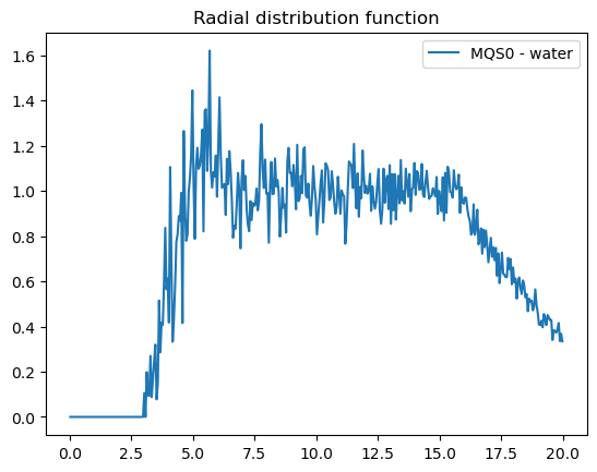
Plot the results

x,y = np.genfromtxt("output/rdf_g000.dat", unpack=True)

plt.title("Radial distribution function")
plt.plot(x,y, label="MQS0 - water")
plt.legend();

Cleanup

for file in glob.glob("output/rdf*"):
    Path(file).unlink() #remove files