![]()
Mean squared displacement
We calculate the mean squared displacement (msd) as well as the msdmj to obtain diffusion and conductivity.
[15]:
import time
import sys
import numpy as np
import matplotlib.pyplot as plt
Some configurations if we are in a google colab environment:
[24]:
IN_COLAB = 'google.colab' in sys.modules
HAS_NEWANALYSIS = 'newanalysis' in sys.modules
if IN_COLAB:
    if not'MDAnalysis' in sys.modules:
        !pip install MDAnalysis
    import os
    if not os.path.exists("/content/mdy-newanalysis-package/"):
        !git clone https://github.com/cbc-univie/mdy-newanalysis-package.git
    !pwd
    if not HAS_NEWANALYSIS:
        %cd /content/mdy-newanalysis-package/newanalysis_source/
        !pip install .
    %cd /content/mdy-newanalysis-package/docs/notebooks/
#if IN_COLAB and not HAS_NEWANALYSIS:
#    !pip install "git+https://github.com/cbc-univie/mdy-newanalysis-package.git@master#egg=newanalysis&subdirectory=newanalysis_source"
Next we import MDAnalysis and functions needed from newanalysis.
[16]:
try:
    import MDAnalysis
except ModuleNotFoundError as e:
    if not IN_COLAB:
        !conda install --yes --prefix {sys.prefix} MDAnalysis
        import MDAnalysis
    else:
        print("Probably the cell above had a problem.")
        raise e
try:
    from newanalysis.diffusion import unfoldTraj, msdCOM, msdMJ
except ModuleNotFoundError as e:
    if not IN_COLAB:
        print("Install newanalysis fist.")
        print("Go to the newanalysis_source folder and run:")
        print("conda activate newanalysis-dev")
        print("pip install .")
    else:
        print("Probably the cell above had a problem.")
    raise e
Preprocessing
Next we create our MDAnalysis Universe:
[17]:
base='../../test_cases/data/emim_dca_equilibrium/'
psf=base+'emim_dca.psf'

skip=20
u=MDAnalysis.Universe(psf,base+"/emim_dca.dcd")
boxl = np.float64(round(u.coord.dimensions[0],4))
dt=round(u.trajectory.dt,4)

n = int(u.trajectory.n_frames/skip)
if u.trajectory.n_frames%skip != 0:
    n+=1
Now we do the selections
[18]:
sel_cat1  = u.select_atoms("resname EMIM")
ncat1     = sel_cat1.n_residues
com_cat1  = np.zeros((n,ncat1,3),dtype=np.float64)
print("Number EMIM   = ",ncat1)

sel_an1  = u.select_atoms("resname DCA")
nan1     = sel_an1.n_residues
com_an1  = np.zeros((n,nan1, 3),dtype=np.float64)
print("Number DCA   = ",nan1)
Number EMIM   =  1000
Number DCA   =  1000
Loop throguh the trajectory and get the center of masses
[19]:
ctr=0
start=time.time()
print("")

for ts in u.trajectory[::skip]:
    print("\033[1AFrame %d of %d" % (ts.frame,len(u.trajectory)), "\tElapsed time: %.2f hours" % ((time.time()-start)/3600))
    com_an1[ctr] = sel_an1.center_of_mass(compound='residues')
    com_cat1[ctr]= sel_cat1.center_of_mass(compound='residues')
    ctr+=1
Frame 0 of 100  Elapsed time: 0.00 hours
Frame 20 of 100         Elapsed time: 0.00 hours
Frame 40 of 100         Elapsed time: 0.00 hours
Frame 60 of 100         Elapsed time: 0.00 hours
Frame 80 of 100         Elapsed time: 0.00 hours
Using newanalysis functions
We now use the unfoldTraj function to undo all jumps due to PBC. This is done in-place.
[20]:
print("unfolding coordinates ..")
unfoldTraj(com_cat1,boxl); #; to suppress output
unfoldTraj(com_an1, boxl);
unfolding coordinates ..
Next we can calculate msd and msdmj
[21]:
print("calculating msd ..")
msd_an1  = msdCOM(com_an1)
msd_cat1 = msdCOM(com_cat1)

#fan1=open("msd_an.dat",'w')
#fcat1=open("msd_cat.dat",'w')

#for i in range(ctr):
#    fan1.write("%5.5f\t%5.5f\n"  % (i*skip*dt, msd_an1[i]))
#    fcat1.write("%5.5f\t%5.5f\n" % (i*skip*dt, msd_cat1[i]))

print("calculating msdMJ ..")
msdmj = msdMJ(com_cat1,com_an1)
#f1=open("msdMJ.dat",'w')
#for i in range(ctr):
#    f1.write("%5.5f\t%5.5f\n" % (i*skip*dt, msdmj[i]))
#f1.close()
calculating msd ..
calculating msdMJ ..
Plot the results
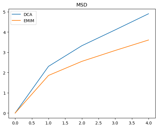
[22]:
time = np.arange(ctr*dt)

plt.title("MSD")
plt.plot(time, msd_an1, label="DCA")
plt.plot(time, msd_cat1, label="EMIM")
plt.legend();
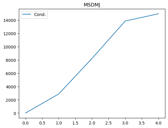
[23]:
plt.title("MSDMJ")
plt.plot(time, msdmj, label="Cond.")
plt.legend();